Switched mode power supplies „SMPS” (Switched Mode Power Supplies)
Switched mode power supplies have replaced traditional linear power supply and are currently the most popular and the largest group of power supplies. Their advantages compared to the linear power supplies are small overall dimensions, low weight, high efficiency and output and low price. The main disadvantages are the complexity of design, high noise generated by the power supply and increased noise level at the output.
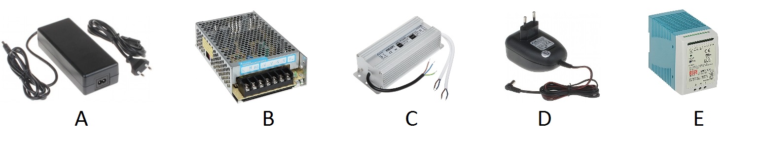
The most common switched mode power supply types:
A - desktop
B - module
C - LED
D - with plug
E - for DIN rail
Basic working principle of switched mode power supply
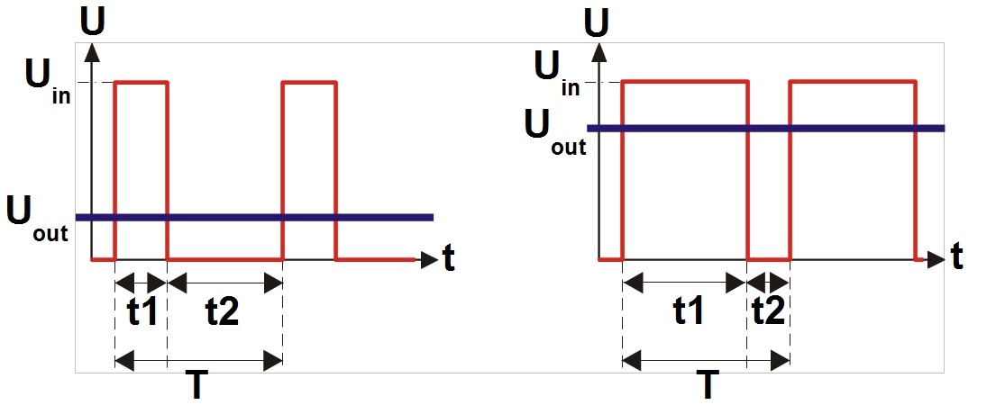
Switched mode power supplies use pulse width modulation PWM (Pulse Width Modulation) technique, i.e. the power supply output voltage is adjusted by changing the duty cycle at constant frequency.
The diagram shows the basic working principle of PWM.
U - voltage
t - time
Uin - input voltage
Uout - output voltage
T - period (periods per seconds is a frequency in Hz, kHz or MHz)
t1 - pulse width (high state)
t2 - no pulse
Reducing the pulse width (t1) reduces the average output voltage (Uout) and vice versa: increasing the pulse width (t1) increases the average output voltage (Uout). As per the graphs:
left - low duty cycle and lower output voltage Uout,
right - high duty cycle and higher output voltage Uout.
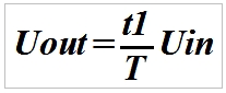
Average output voltage can be easily calculated from the following equation:
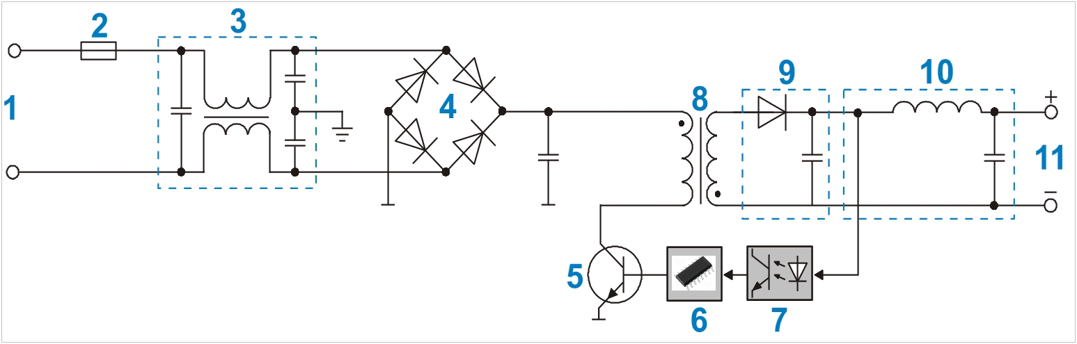
Diagram and basic working principle of switched mode power supply:
1 - AC voltage input
2 - fuse
3 - input filter
4 - rectifier unit (diode bridge)
5 - keying transistor
6 - PWM controller
7 - optical coupler (galvanic isolator)
8 - peaking transformer
9 - rectifier
10 - output filter
11 - DC voltage output
Alternating mains voltage, e.g. 230 V (1) passes through the LC input filter (3). Input filter is a key component protecting the mains against noise generated by the power supply and protecting the power supply against noise generated by the mains. The alternating voltage is rectified by a bridge rectifier (4) and as a constant voltage is fed to the transformer (8), keyed by a transistor (5) also referred to as a switch. The transistor activates and deactivates a rectangular waveform current at a specific frequency (20 kHz to several hundred kHz or even MHz), using the pulse width modulation (PWM) technique. The transistor is controlled by a feedback system (6, 7) including an optical coupler and a PWM controller. The system verifies the output voltage and changes the impulse width (duty cycle) depending if the voltage increases or decreases via a transistor to adjust the voltage to a constant value. The system verifies the output voltage with high speed to maintain the constant output voltage and compensate any changes to maintain the constant level. A rectangular waveform voltage at the transformer output (8) is rectified (9) and passes through the output filter (10) which blocks higher harmonics and noise generated by the converter. Stabilized constant voltage is generated at the output (11) of the switched mode power supply.
The following parameters should be considered when selecting the switched mode power supply.
Input Voltage
In Poland and other EU countries the mains voltage is 230 V AC (except for UK - 240 V AC). The standards allow 10% deviation, i.e. the mains voltage can fluctuate from 207 to 253 V AC. Thus, a power supply with a wide range of input voltage, e.g. 100–264 V AC is recommended.
Max Inrush Current
Large current pulse is generated at power on that, depending on the power, may reach high values up to tens of amperes with a duration of up to one period, i.e. up to 20 ms at 50 Hz AC. This phenomenon is caused by input capacitor charging and may be problematic when powering on several power supplies or using high power devices. High starting current can trip the mains protection (fuses, overcurrent circuit breaker etc.). The problem can be resolved by using type C or type D overcurrent circuit breakers.
Efficiency
It is a ratio of the DC output power (generated by the power supply) to AC input power (received from the mains) expressed as percentages.
The efficiency is typically denoted by the Greek small letter eta: η. In all devices converting the energy, part of the input power is lost and the efficiency is a measure of power loss. This parameter is noteworthy, since the higher the efficiency, the less energy is lost which means that the temperature inside the power supply is lower and as a result, the reliability and service life are increased. Available switched mode power supplies offer efficiencies >90% (transformer or linear power supplies efficiency does not exceed 50%).
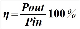
Efficiency formula:
η – efficiency (%)
Pout – output power
Pin - input power
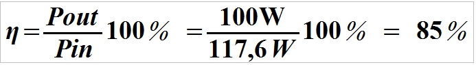
Example 1. The efficiency of a power supply with 100 W output power at mains power input of 117.6 W can be calculated as follows:
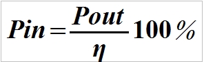
In the data sheets, the manufacturers usually specify output power and efficiency of the power supply, however, the power input is not usually specified. It can be easily calculated using the following equation.
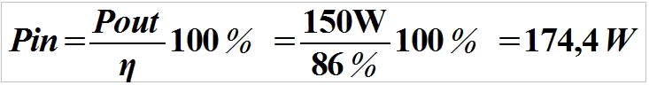
Example 2. Power supply with 150W output power and 86% efficiency. Mains power input can be calculated as follows:
Power loss as a thermal energy (Pd – power loss) can be calculated using a simple equation (take away the generated power from the power input).
In this case, 24.4 W is lost as a thermal energy at full load. Those 24.4 W increase the temperature inside the enclosure and the temperature of internal components.
MTBF - Mean Time Between Failure
It is expressed in hours and indicate the reliability of the device.
This parameter is often misinterpreted. MTBF of the power supply may be 700,000 hours, i.e. almost 80 years. However, it does not mean that the power supply will operate failure-free for such a long time.
The methods to calculate MTBF were introduced by the US Army in 1965 with the publication of MIL-HDBK-217 model. The model included the failure rates for different electronic components, i.e. capacitors, resistors and transistors and the methods to calculate the failure rate. It was supposed to standardise the reliability evaluation methods for electronic and military equipment.
Apart from MIL-HDBK-217 models, other models to calculate the MTBF are available in the specifications for electronic devices. The models use different algorithms to calculate reliability. Example methods: HRD5, Telcordia, RBD, Markow model, FMEA/FMECA, failure tree, HALT.
With a known MTBF time we can calculate the probability of the device failure before the MTBF elapses. It is a very useful information that allows to evaluate the overall reliability of a system. The rule is simple: the higher the MTBF, the more reliable the device.
MTBF is a time, after which the reliability of the device drops to 36.8%.
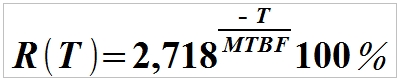
How is that possible? The calculation uses an equation for reliability.
R(T) – reliability expressed as percentages in relation to device operation time
T – device operation time
MTBF – mean time between failure
2,718 – Euler number (denoted as the letter "e")
In words: 2,718 to the negative power of operation time divided by MTBF.
Let us calculate the failure rate of a device with MTBF of 50,000 hours after 50,000 hours of operation.
The device with MTBF = 50,000 hours has a reliability of 36.8% after 50,000 hours of operation. In other words, after 50,000 hours, the probability is that for every 100 devices approx. 37 will still be in operation and 63 will fail.
Let us verify the probability of a failure within 3 years for two power supplies with different MTBF.
1. MTBF = 50,000 hours, 3 years = 3 years x 24 hours x 365 days = 26,280 hours:
The results show the probability that after 3 years 59.1% of the power supplies will still be in operation (e.g. for every 100 devices, approx. 59 devices will still be in operation and 41 will fail).
2. MTBF = 70,000 hours, 3 years = 3 years x 24 hours x 365 days = 26,280 hours:
This case shows the probability that after 3 years 97.1% of the power supplies will still be in operation (e.g. for every 100 devices, approx. 97 will still be in operation and 3 will fail).
Most often, MTBF is determined by the manufacturer in relation to the device operation at 25°C. For operation at higher temperatures, the increase in temperature by 10°C reduces the MTBF by half. Why does MTBF differ for different devices? The difference is usually due to the quality of components and the degree of complexity. Not all manufacturers include this parameter in the product specification.
Output Voltage
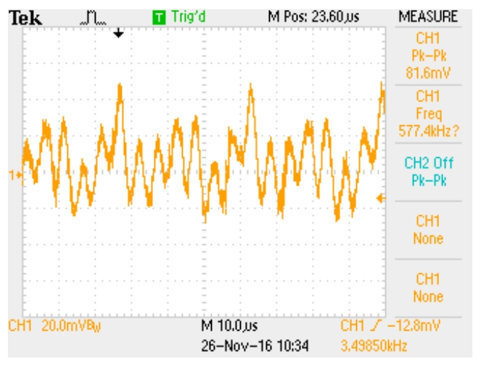
The output voltage is the voltage that must be stabilised at changes in power supply load from 0 to 100%. Remember, that the output voltage for all power supplies includes noise, ripples and interferences with an amplitude reaching up to several hundred mVp-p. High output voltage ripple may cause problems if the supplied device is susceptible to ripples, e.g. interferences in the images recorded by CCTV cameras or frequent restarts of electronic devices.
An example oscillogram of a 12V switched mode power supply voltage ripples is shown below.
Dynamic Response
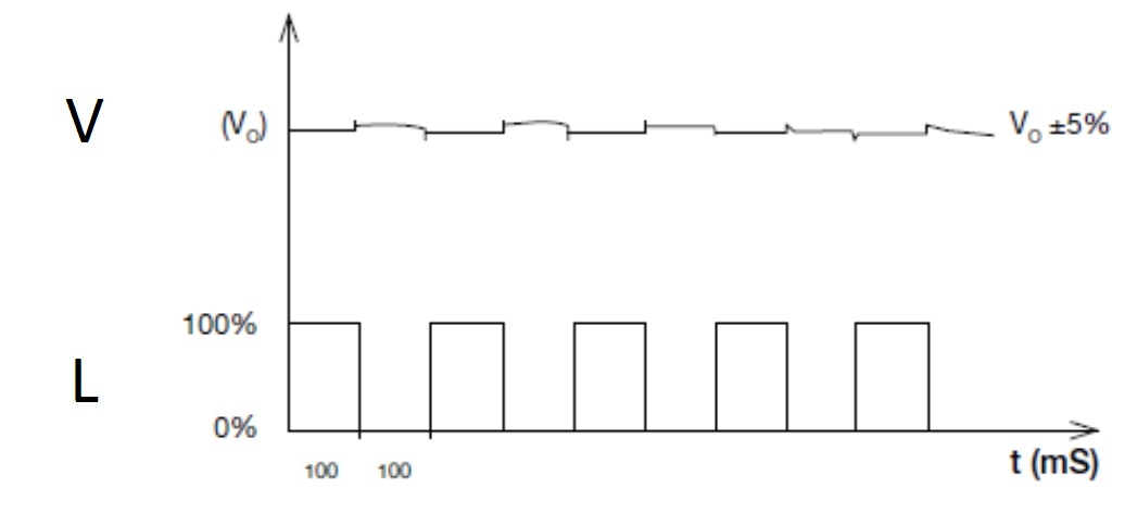
Each power supply should deliver constant output voltage irrespective of the changes in load current. However, load variations may occur (e.g. switching the IR illuminator in the CCTV camera or the auxiliary load). The load variation from 0 to 100% or vice versa may introduce interferences and output voltage fluctuations that may affect operation of other devices connected to the power supply.
The diagram shows changes in the output voltage due to changes in load from 0 to 100% for a high-quality power supply from (based on the specification).
V - output voltage
L - load
Most switched mode power supplies are fitted with protections against short-circuit and overload. Since different protections are used, the power supply must be suitable to the load type. Motors, incandescent bulbs, high capacity and high inductance loads etc., i.e. loads with non-linear characteristics may require high current pulse at power on exceeding the maximum rated current of the power supply. It may trip the protection and prevent the power supply from starting. In practice, a 12V 50W power supply will not be able to supply a 12V 30W load (e.g. incandescent light bulb or motor).
The designers of power supplies use different methods to prevent short circuits and overloads. The protection should guarantee safety of both the power supply and the load. The most commonly used protections are discussed below.
Hiccup mode
It is one of the most commonly used protections hiccup characterised by low power loss in the power supply due to overload or short circuit and automatic restoration of normal operation after the cause of the short circuit or overload has been eliminated.
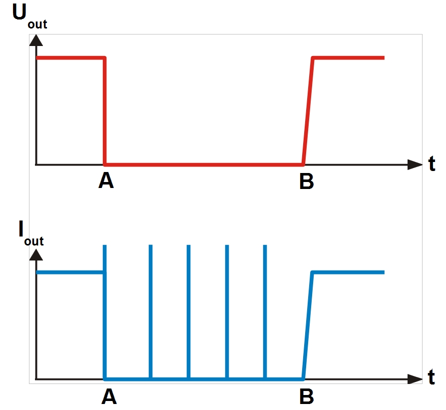
The diagram below shows the basic working principle of hiccup type protection.
Uout - output voltage
Iout - output current
t - time
A – short-circuit (overload)
B – short-circuit cause eliminated
Overload or short-circuit take place at A. Power supply is disconnected. Very short duration current pulse (e.g. 100 ms) at 150% maximum current is generated at the output. The power supply will transmit this pulse every several seconds until the cause for overload or short-circuit (B) is eliminated and restores normal operation mode. In most cases, the activation threshold (power supply disconnection) is set to 110 to 150% rated current (Iout). This mode is usually integrated with a thermal protection. If the load requires current higher than the rated current but lower than the threshold, the thermal protection will be activated after a while to disconnect the power supply and switch to hiccup mode until the cause for the overload is eliminated.
Other types of protections against high current input are shown below (3 curves: A, B and C).
Uout - output voltage
Iout - output current
Curve A – foldback current limiting (Foldback Current Limiting) This type of protection is also used in linear power supplies. After the maximum current is exceeded (reduced load resistance), the current is reduced. In other words, if the load resistance is reduced the current is also reduced. This method is characterized by low power loss at the power supply in case of an overload or short-circuit. However, the power supply will not start with loads that require high starting currents (e.g. high capacity loads).
Curve B – constant current limiting (Constant Current Limiting) After exceeding the maximum current (reduced load resistance), the power supply maintains constant output current regardless of the overload simultaneously reducing the output voltage. Auxiliary protection disconnecting the power supply in case the voltage drops to several volts is often used. This method is characterized by large power losses at the power supply and high current flow through the load that may result in damage. This type of protection allows to start a power supply with non-linear loads connected.
Curve C – overpower limiting (Over Power Limiting) After the maximum current is exceeded (reduced load resistance), the output power of the power supply is maintained at a constant level. With the increase in load, the voltage and the output current drop in accordance with the C curve. This type of protection allows to start a power supply with non-linear loads connected.
Working Temperature, Surrounding Air Temperature
Depending on the power supply efficiency, part of the energy supplied to the power supply is lost as thermal energy, the temperature inside the power supply increases in relation to the external temperature. High quality power supplies operating at 25°C may heat up to 50-70°C. At ambient temperature of 50°C, the temperature of a power supply may reach up to 75-95°C.
The operating temperature directly affects the service life and reliability of the device. Switched mode power supplies are very complex and consists of a large number of electronic components that may be arranged close to each other inside the enclosure. High ambient temperature may lead to damage and significantly reduce service life. There is a strong correlation between the output power and the temperature. Avoid power supply operation at temperatures exceeding 50°C despite the fact that the manufacturers often specify higher operating temperatures. Carefully read the device specifications.
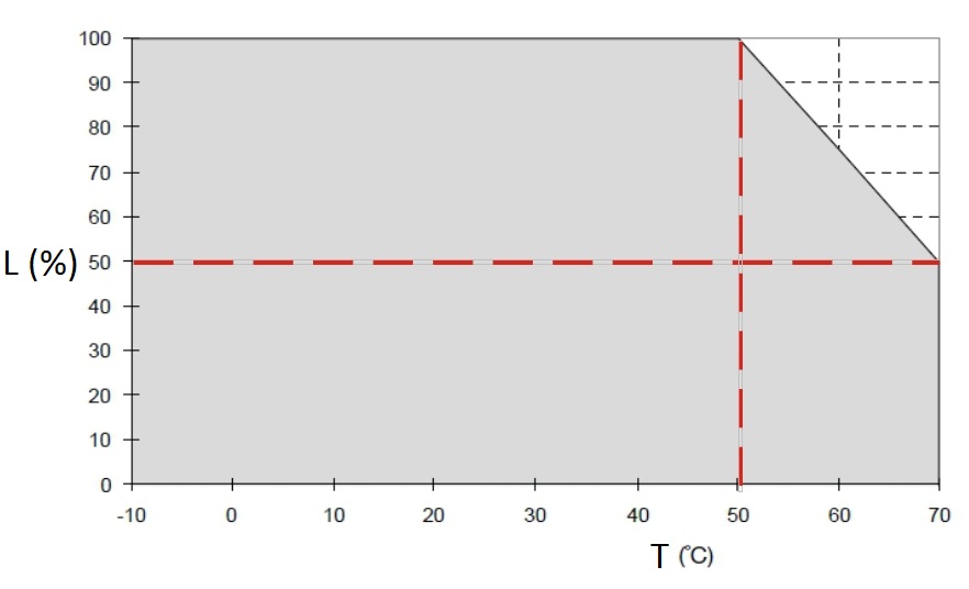
For example, the operating temperature for a 150W 12V power supply is -10°C to 70°C. However, the specification includes a graph of percentage load as a function of operating temperature.
L - Percentage of Max Load
T - Surrounding Air Temperature
The graph shows that the device can supply full power up to 50°C. At 70°C, the device can supply 50% of the maximum current.
Electrolytic capacitors used in almost every single power supply are the components most sensitive to an increase in temperature. The capacitor manufacturers include a key parameter, i.e. service life at maximum operating temperature. Decreasing the temperature by 10°C will double the service life of the electrolytic capacitor. For example, the service life of a standard electrolytic capacitor is 1,000 hours at 105°C.
I.e.:
105°C – 1,000 hours (41 days)
95°C – 2,000 hours (83 days)
85°C – 4,000 hours (83 days)
75°C – 8,000 hours (166 days)
65°C – 16,000 hours (1.8 years)
55°C – 32,000 hours (3.6 years)
45°C – 64,000 hours (7.3 years)
The service life does not necessary mean that the capacitor will fail, however, its performance will be significantly reduced (capacity, serial resistance etc.) which may lead to failure.
The lower the temperature the longer the service life. Capacitors with a service life several times longer are available, however, those are much more expensive. Its the manufacturer who decides on the components used. More expensive components with a longer service life are not usually used in less expensive power supplies.
Net:
0.00
EUR
Gross:
0.00
EUR
Weight:
0.00
kg
This site uses cookies. More information about using by us cookie files, their usage and how to modify the acceptance of cookie files, can be found by pressing
link
 English
 Български
 Český
Český Dansk
Dansk Deutsch
 Eesti
Eesti Ελληνικά
 Español
 Français
 Italiano
 Latviešu
  Lietuvių
  Magyar
 Nederlands
 Polski
 Português
 Pусский
 Română
 Slovenski
 Slovenský
 Suomi
Suomi Svenska
 EUR
EUR AUD
AUD CAD
CAD CHF
CHF CZK
CZK DKK
DKK GBP
GBP HUF
HUF NOK
NOK PLN
PLN SEK
SEK USD
USD
 Home
Home Contact
 New products